In industries where sales are a major focus, keeping track of when you last contacted or visited clients is essential. Maintaining a sales log can help automatically update the list of clients with their last visit date or the number of days since their last visit.
In this guide, we will learn how to calculate the number of days since the last visit to a client using the DATEDIF and VLOOKUP functions. Typically, sales logs and client sheets are managed separately, but for simplicity, we will work on a single sheet in this example.
Setting Up Calculating Days Since Last Client Visit

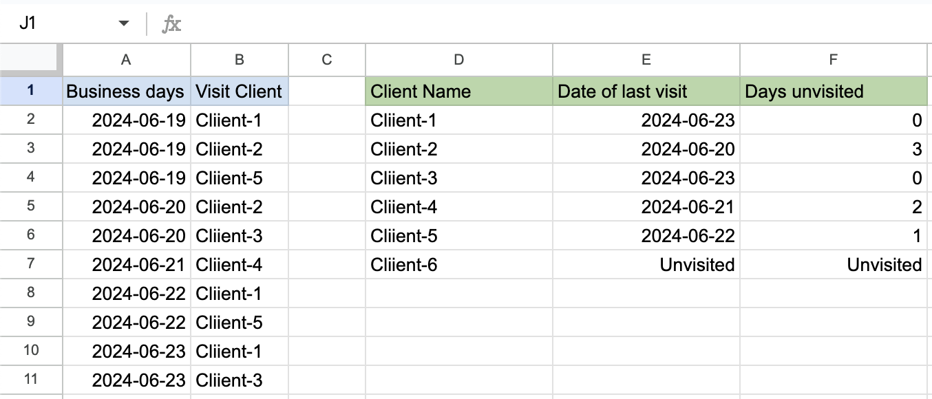
Let’s assume you have a sales log on the left side of your sheet and a client sheet on the right. While the sales log can contain various details like sales content and the person in charge, and the client sheet can have details like phone numbers, contact names, addresses, and business registration numbers, we will focus on the sales date and the number of days since the last visit.
Creating a Sales Log and Client Sheet:
- Sales Log (Columns A and B):
- Column A: Business days
- Column B: Visit Client
- Client Sheet (Columns D and E and F):
- Column D: Client Names
- Column E: Date of last visit (calculated using VLOOKUP)
- Column F: Days unvisited (calculated using DATEIF & VLOOKUP)
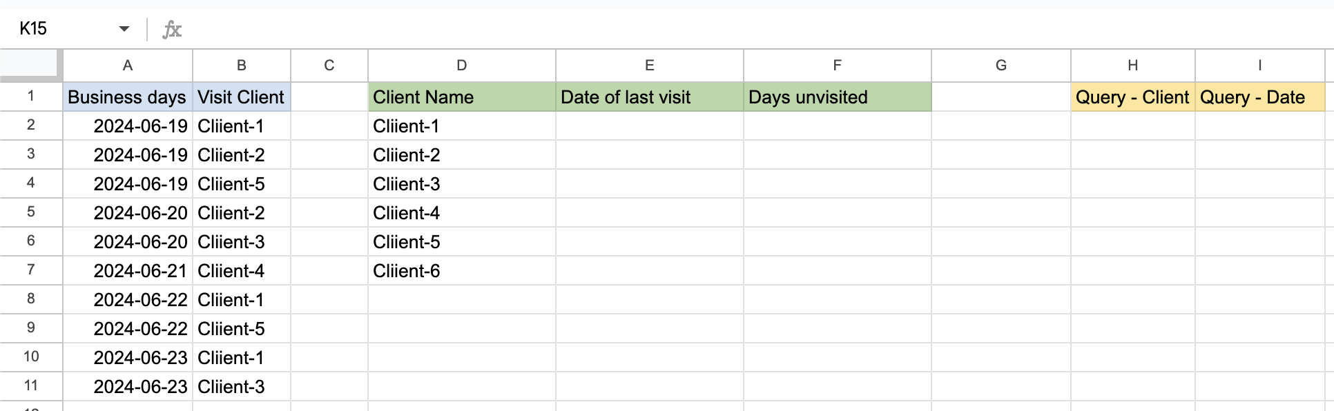
- Client Sheet (Columns H and I):
- Column H: Query – Client
- Column I: Query – Date
Identify the Last Visit Date Using QUERY:
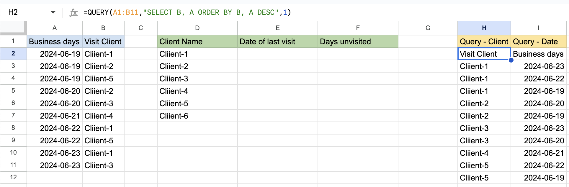
To find the last visit date for each client, we need to sort the sales log by client name and date in descending order. This can be done using the QUERY function.
QUERY(A1:B11, "SELECT A, B ORDER BY A, B DESC", 1)This query sorts the data by client name and then by sales date in descending order. The result will look something like this
| Client Name | Sales Date |
|---|---|
| Client1 | 2024-06-23 |
| Client1 | 2024-06-22 |
| Client1 | 2024-06-19 |
| Client2 | 2024-06-20 |
| Client2 | 2024-06-19 |
| Client3 | 2024-06-23 |
Creating reference areas with Named ranges
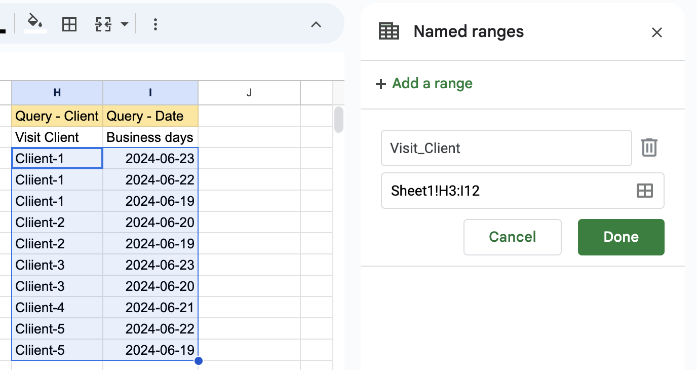
Name the range of the query result for easier reference. (name = Visit_Client, Range = Sheet1!H3:H12)
Use VLOOKUP to Find the Last Visit Date
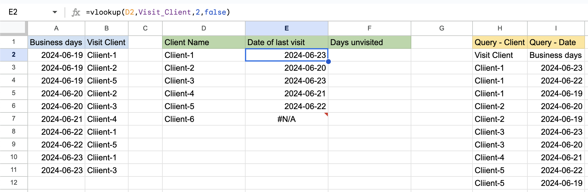
Next, we use VLOOKUP to find the last visit date for each client
- Select the range of the QUERY result and name it
Visit_Client.
=VLOOKUP(D2, Visit_Client, 2, FALSE)This formula looks up the client name in D2 within the Visit_Client
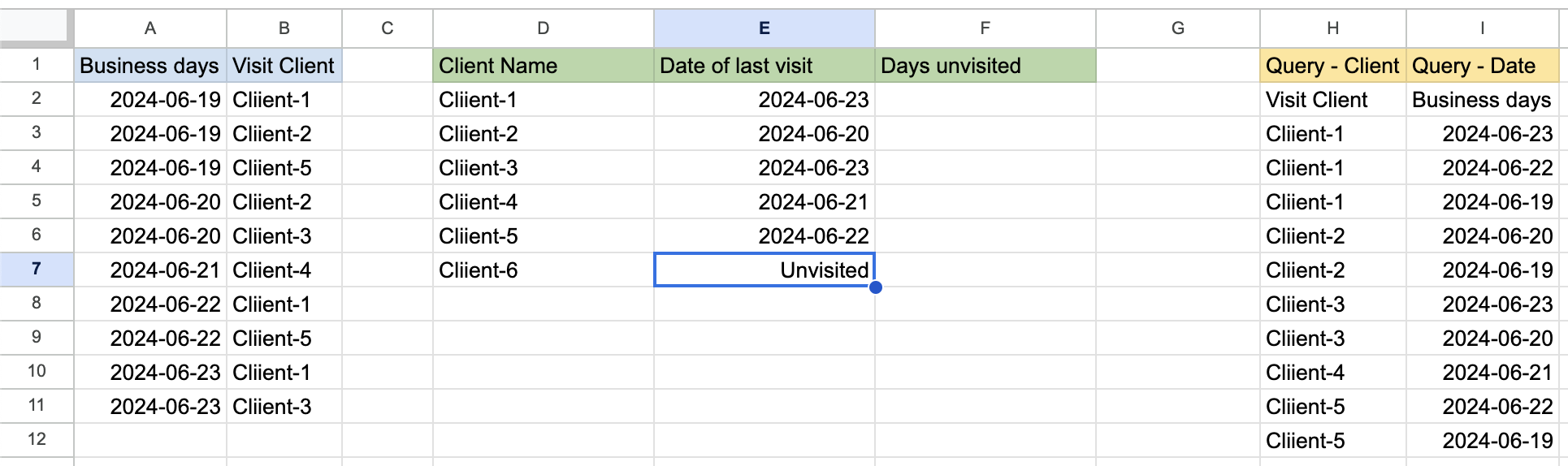
Modify the existing function by adding “IFNA” to display the value as “Unvisited” if it is displayed as N/A because there is no matching date.
=IFNA(VLOOKUP(D2,Visit_Client,2,false),"Unvisited")Calculate Days Since Last Visit Using DATEDIF
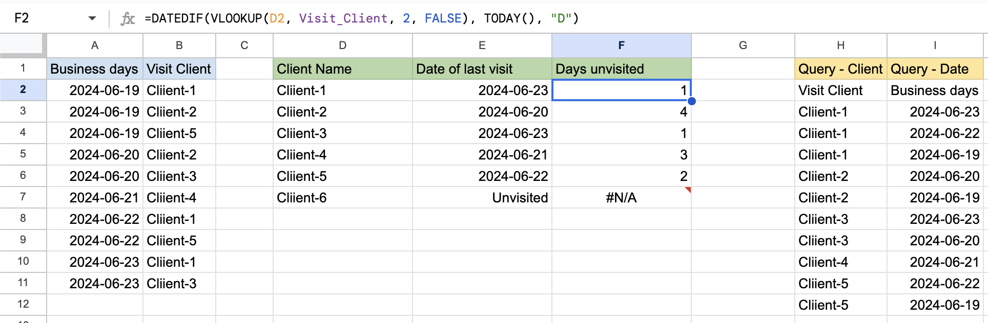
Finally, we use the DATEDIF function to calculate the number of days since the last visit. The formula is as follows
=DATEDIF(VLOOKUP(D2, LastVisitData, 2, FALSE), TODAY(), "D")This formula calculates the difference in days between today’s date and the last visit date obtained from the VLOOKUP function.
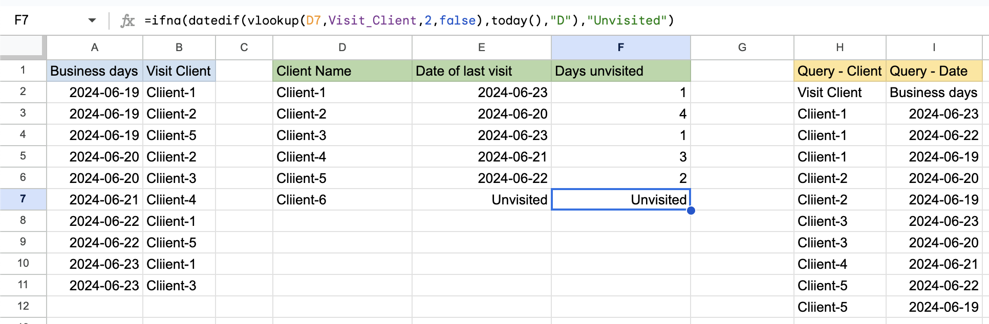
Modify the existing function by adding “IFNA” to display the value as “Unvisited” if it is displayed as N/A because there is no matching date.
=IFNA(DATEDIF(VLOOKUP(D7,Visit_Client,2,false),today(),"D"),"Unvisited")Additional Notes
- QUERY Function: The
QUERYfunction in Google Sheets allows you to perform queries similar to SQL. In this case, we use it to sort the data by client name and sales date. - VLOOKUP Function: The
VLOOKUPfunction searches for a value in the first column of a range and returns a value in the same row from a specified column. TheFALSEargument ensures an exact match. - DATEDIF Function: The
DATEDIFfunction calculates the difference between two dates. The “D” argument specifies that the difference should be returned in days.
By following these steps, you can automate the calculation of days since the last visit for each client, making your sales tracking more efficient and accurate.
For more detailed information on using Named ranges and Data validation rules, visit the official website here.
For more information on how to do more with Google Sheets, see this guide.
> Mastering Spreadsheets: Extracting Unique Data Using FILTER and MATCH
> Mastering Spreadsheets: Highlighting Duplicate Entries with Conditional Formatting
> Mastering Spreadsheets: Named ranges + Data validation rules = Perfect
> Mastering spreadsheets: Goal seek(with PMT)
> How to Create a Line Chart in Google Sheets: A Beginner’s Guide
> Google Sheets Org Chart Guide: A Beginner-Friendly Tutorial
#Google Sheets #QUERY #DATEDIF #VLOOKUP