When working with data, you may encounter situations where you need to compare two columns and extract only the unique entries. This often occurs when dealing with automatically generated data and manually entered data. For example, you might need to extract new clients from a list, excluding those already existing in your records.
Function Overviews: FILTER, MATCH, ISNA
FILTER
The FILTER function extracts data that meets specified criteria.
Usage:
FILTER(range, condition1, [condition2, ...])
Example:
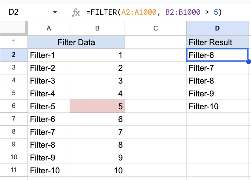
=FILTER(A2:A1000, B2:B1000 > 5)
This filters the range A2 to show only the cells where the corresponding B2cells are greater than 5.
MATCH
The MATCH function searches for a specified item in a range and returns its relative position.
Usage:
MATCH(search_key, range, [match_type])
Example:
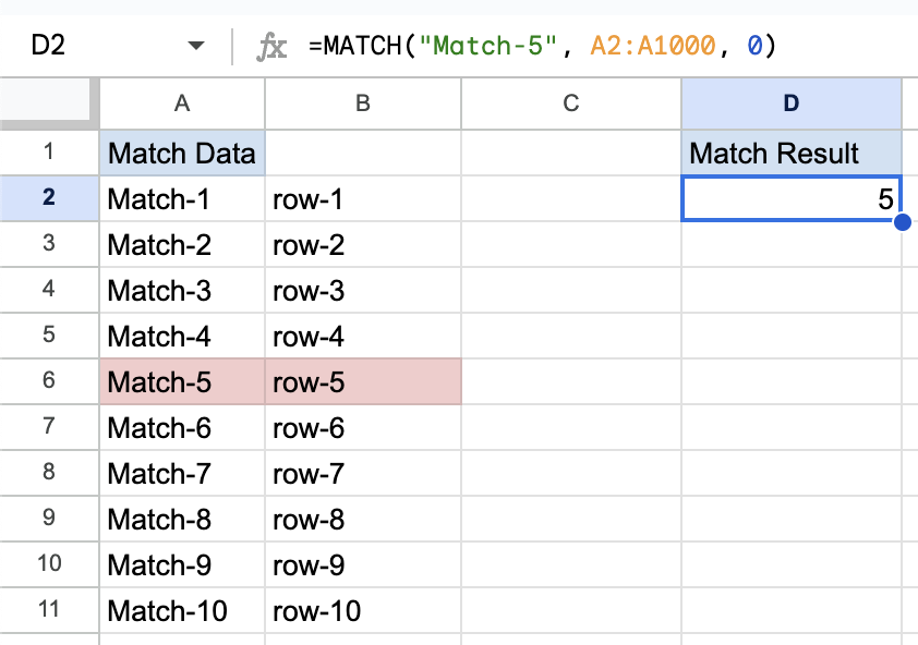
=MATCH("Match-5", A2:A1000, 0)
This returns the position of “Match-5” within the range A2. The match_type 0 indicates an exact match.
ISNA
The ISNA function checks if a value is the error #N/A and returns TRUE or FALSE.
Usage:
ISNA(value)
Example:
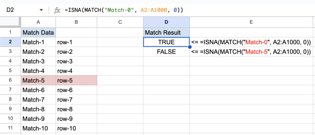
=ISNA(MATCH("Match-0", A2:A1000, 0))
This returns TRUE if “Match-0Match-
Setting Up Extracting Unique Data

Let’s use these functions to find unique clients in a list.
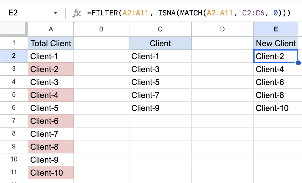
Scenario: You have a list of 10 clients (automatically generated) in column A. Out of these, 5 are already existing clients (manually entered) in column C. You need to extract the 5 new clients.

Formula:
=FILTER(A2:A11, ISNA(MATCH(A2:A11, C2:C6, 0)))
Explanation:
- Purpose: Extract values in A2that do not appear in C2.
- Filter Function:
FILTER(A2:A11, condition)extracts values from A2based on a condition. - Condition:
ISNA(MATCH(A2:A11, C2:C6, 0))checks if values in A2are not found in C2.
Let’s break down the condition:
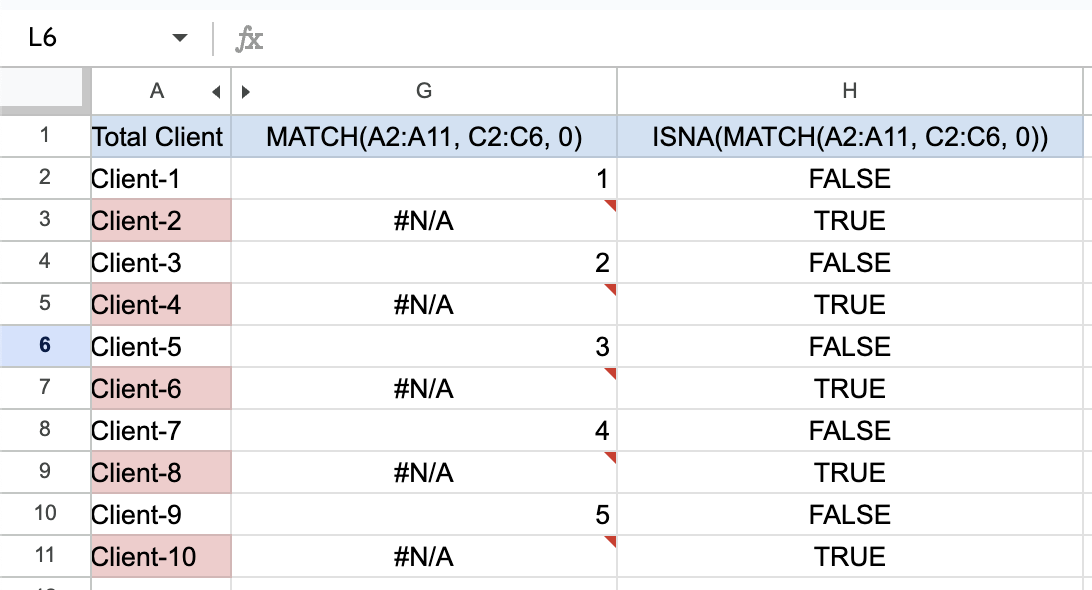
- MATCH(A2:A11, C2:C6, 0): Finds the position of each value in A2:A11 within C2:C6. If a value is not found, it returns
#N/A. - ISNA(…): Checks if the result of MATCH is
#N/A, indicating the value is unique to A2.
Additional Notes: ARRAYFORMULA
The ARRAYFORMULA function enables array calculations on ranges, allowing functions that typically work on single cells to be applied to ranges.
Usage:
ARRAYFORMULA(function(range))
Example:
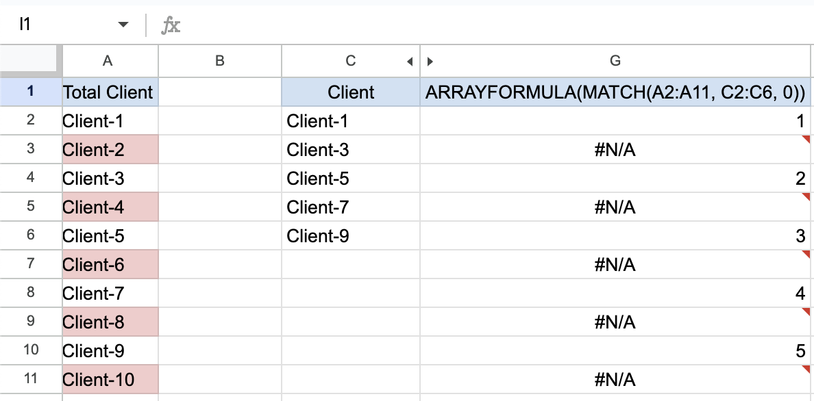
=ARRAYFORMULA(MATCH(A2:A11, C2:C6, 0))
This applies the MATCH function across the entire range A2.
Practical Application
In practice, you can use this method to manage various datasets, such as generating lists of invoices to issue by excluding those already issued.
Example Use Case
You have a list of invoices to be issued and a list of already issued invoices. By using the above method, you can extract the list of pending invoices.
Try this approach on your dataset and see how it simplifies data management. Remember, these functions are powerful tools to keep your data organized and error-free.
For more detailed information on using Named ranges and Data validation rules, visit the official website here.
For more information on how to do more with Google Sheets, see this guide.
> Mastering Spreadsheets: Highlighting Duplicate Entries with Conditional Formatting
> Mastering Spreadsheets: Named ranges + Data validation rules = Perfect
> Mastering spreadsheets: Goal seek(with PMT)
> How to Create a Line Chart in Google Sheets: A Beginner’s Guide
> Google Sheets Org Chart Guide: A Beginner-Friendly Tutorial
#Google Sheets #Google Sheets Named ranges #Google Sheet Data validation