In managing unique data such as clients or products, spotting duplicate entries can be straightforward when dealing with small datasets. However, as the number of entries grows, manually identifying duplicates or using pivot tables becomes cumbersome. Conditional formatting offers an efficient solution by visually highlighting duplicate cells, allowing you to quickly identify issues and receive immediate feedback upon data entry.
Setting Up Conditional Formatting

Example Scenario: Highlighting Duplicate Car Models
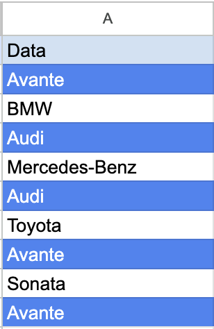
Suppose you have a list of car models in column A and you want to highlight any duplicates.
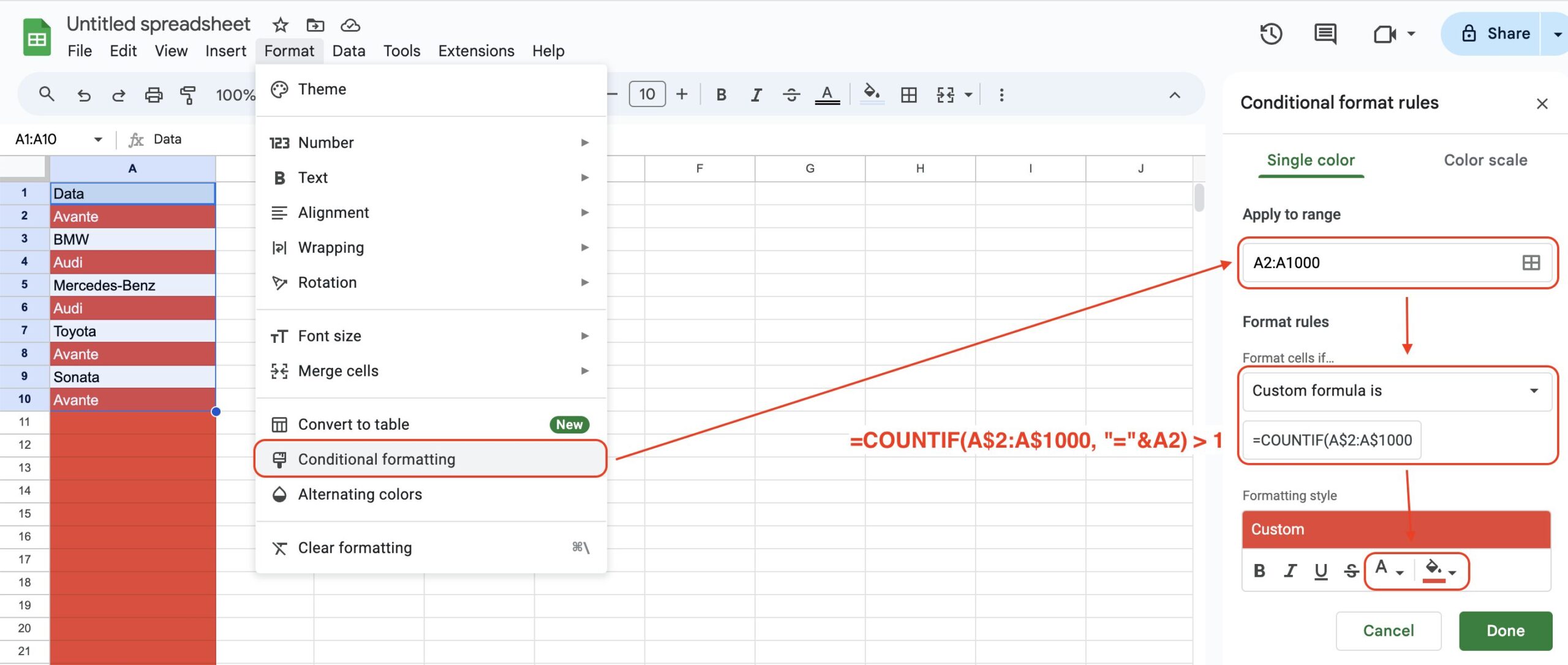
- Select the Range for Conditional Formatting: Begin by selecting the range of cells where you want to apply conditional formatting. Click on the tool bar “Format” and choose “Conditional Formatting”.
- Adjusting the Range: If you want to apply this rule to an entire column, set the range to A4. This ensures the rule covers all potential entries up to row 1000. Change the formatting color to red for better visibility.
- Setting Up the Custom Formula: Choose “Custom formula is” from the format rules.
=COUNTIF(A$2:A$1000, "="&A2) > 1This formula counts the occurrences of the value in A within the range A2. If the count exceeds 1, it means a duplicate is present, and the conditional formatting is applied.
Key Points for the Formula:
- The formula must start with an
=sign. - Use absolute referencing (
$) for the row numbers to ensure the formula correctly applies to all cells in the range. - Enclose the condition in
COUNTIFwithin quotes (" "), and use&to concatenate the condition with the cell value being checked (A2 in this case).
Avoiding False Positives from Blank Cells
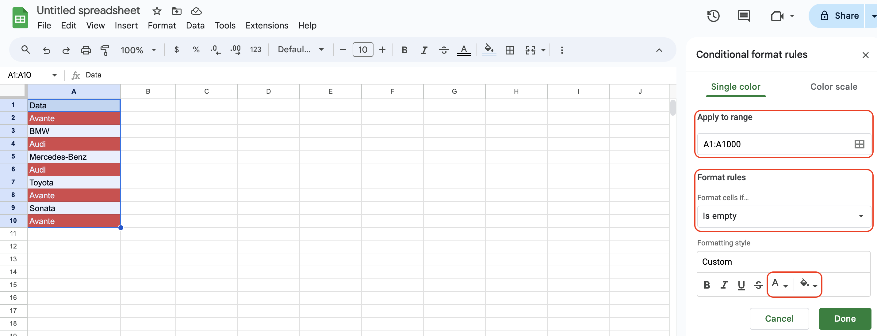
Blank cells may also be highlighted as duplicates, which can be visually unappealing. To prevent this, add another conditional formatting rule to ignore blank cells. (Add another rule)
- Set the Rule for Blank Cells: Choose “Is empty”
- Set the formatting to no color or white to ensure these cells are not highlighted.
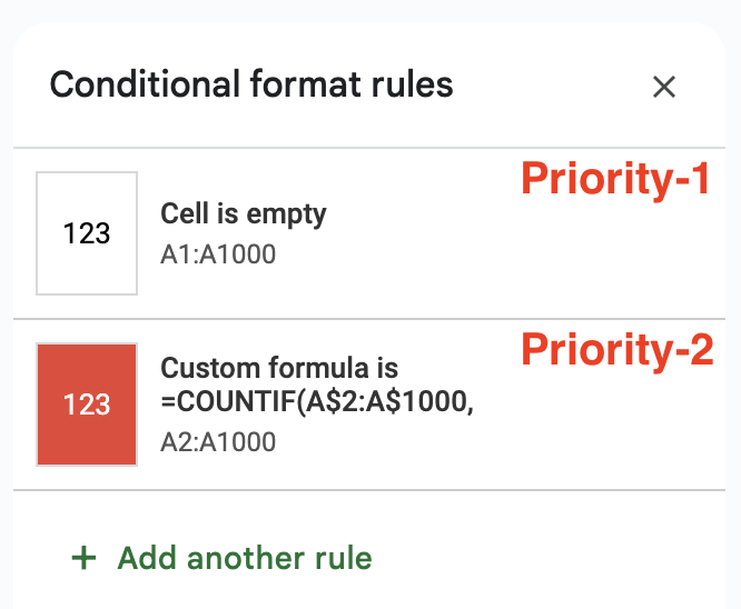
Order the Rules: Make sure the rule for blank cells is placed above the rule for duplicates in the conditional formatting rules list. Conditional formatting rules are applied in order, and this ensures that blank cells remain unaffected by the duplicate highlighting rule.
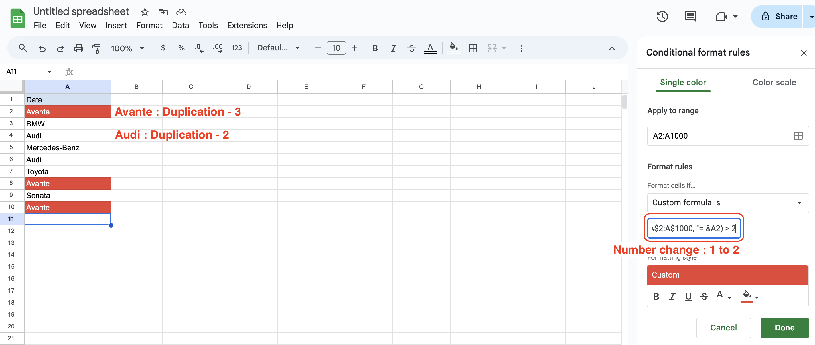
If you want to find three or more duplicate values instead of two or more, just change the value in formula.
=COUNTIF(A$2:A$1000, "="&A2) > 2Conclusion
After applying these rules, any duplicate entries within the specified range will be highlighted in red, excluding blank cells. This makes it easier to manage and verify unique entries in your dataset, enhancing the accuracy of your data analysis.
Implementing conditional formatting to highlight duplicates in your spreadsheets is a powerful way to maintain data integrity. It simplifies the process of identifying and correcting duplicate entries, making your data management more efficient and reliable.
For more detailed information on using Named ranges and Data validation rules, visit the official website here.
For more information on how to do more with Google Sheets, see this guide.
> Mastering Spreadsheets: Named ranges + Data validation rules = Perfect
> Mastering spreadsheets: Goal seek(with PMT)
> How to Create a Line Chart in Google Sheets: A Beginner’s Guide
> Google Sheets Org Chart Guide: A Beginner-Friendly Tutorial
#Google Sheets #Google Sheets Named ranges #Google Sheet Data validation